Iteration Space Coloring: Mesh Vertex Sum
This section contains an exercise file RAJA/exercises/vertexsum-indexset.cpp
for you to work through if you wish to get some practice with RAJA. The
file RAJA/exercises/vertexsum-indexset_solution.cpp contains complete
working code for the examples discussed in this section. You can use the
solution file to check your work and for guidance if you get stuck. To build
the exercises execute make vertexsum-indexset and make vertexsum-indexset_solution
from the build directory.
Key RAJA features shown in this example are:
RAJA::forallloop execution template method
RAJA::TypedListSegmentiteration space construct
RAJA::TypedIndexSetiteration space segment container and associated execution policies
The example computes a sum at each vertex on a logically-Cartesian 2D mesh as shown in the figure.
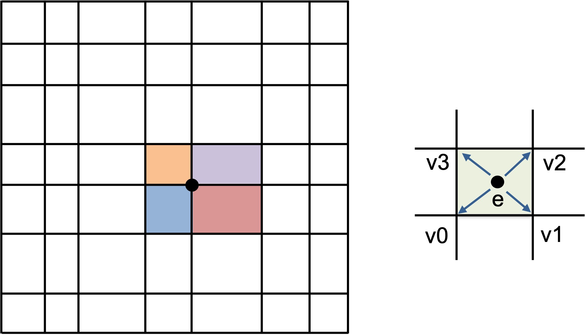
The “area” of each vertex is the sum of an area contribution from each element sharing the vertex (left). In particular, one quarter of the area of each mesh element is summed to the vertices surrounding the element (right).
Each sum is an average of the area of the four mesh elements that share the vertex. In many “staggered mesh” applications, an operation like this is common and is often written in a way that presents the algorithm clearly but prevents parallelization due to potential data races. That is, multiple loop iterates over mesh elements may attempt to write to the same shared vertex memory location at the same time. The example shows how RAJA constructs can be used to enable one to express such an algorithm in parallel and have it run correctly without fundamentally changing how it looks in source code.
We start by setting the size of the mesh, specifically, the total number of elements and vertices and the number of elements and vertices in each direction:
//
// 2D mesh has N^2 elements (N+1)^2 vertices.
//
  constexpr int N = 1000;
  constexpr int Nelem = N;
  constexpr int Nelem_tot = Nelem * Nelem;
  constexpr int Nvert = N + 1;
  constexpr int Nvert_tot = Nvert * Nvert;
We also set up an array to map each element to its four surrounding vertices and set the area of each element:
//
// Define mesh spacing factor 'h' and set up elem to vertex mapping array.
//
  constexpr double h = 0.1;

  for (int ie = 0; ie < Nelem_tot; ++ie) {
    int j = ie / Nelem;
    int imap = 4 * ie ;
    e2v_map[imap] = ie + j;
    e2v_map[imap+1] = ie + j + 1;
    e2v_map[imap+2] = ie + j + Nvert;
    e2v_map[imap+3] = ie + j + 1 + Nvert;
  }

//
// Initialize element areas so each element area
// depends on the i,j coordinates of the element.
//
  std::memset(areae, 0, Nelem_tot * sizeof(double));

  for (int ie = 0; ie < Nelem_tot; ++ie) {
    int i = ie % Nelem;
    int j = ie / Nelem;
    areae[ie] = h*(i+1) * h*(j+1);
  }
Then, a sequential C-style version of the vertex area calculation looks like this:
  std::memset(areav_ref, 0, Nvert_tot * sizeof(double));

  for (int ie = 0; ie < Nelem_tot; ++ie) {
    int* iv = &(e2v_map[4*ie]);
    areav_ref[ iv[0] ] += areae[ie] / 4.0 ;
    areav_ref[ iv[1] ] += areae[ie] / 4.0 ;
    areav_ref[ iv[2] ] += areae[ie] / 4.0 ;
    areav_ref[ iv[3] ] += areae[ie] / 4.0 ;
  }
We can’t parallelize the entire computation at once due to potential race conditions where multiple threads may attempt to sum to a shared element vertex simultaneously. However, we can parallelize the computation in parts. Here is a C-style OpenMP parallel implementation:
  std::memset(areav, 0, Nvert_tot * sizeof(double));

  for (int icol = 0; icol < 4; ++icol) {
     const std::vector<int>& ievec = idx[icol];
     const int len = static_cast<int>(ievec.size());

     #pragma omp parallel for
     for (int i = 0; i < len; ++i) {
        int ie = ievec[i];
        int* iv = &(e2v_map[4*ie]);
        areav[ iv[0] ] += areae[ie] / 4.0 ;
        areav[ iv[1] ] += areae[ie] / 4.0 ;
        areav[ iv[2] ] += areae[ie] / 4.0 ;
        areav[ iv[3] ] += areae[ie] / 4.0 ;
     }

  }
What we’ve done is broken up the computation into four parts, each of which can safely run in parallel because there are no overlapping writes to the same entry in the vertex area array in each parallel section. Note that there is an outer loop on length four, one iteration for each of the elements that share a vertex. Inside the loop, we iterate over a subset of elements in parallel using an indexing area that guarantees that we will have no data races. In other words, we have “colored” the elements as shown in the figure below.
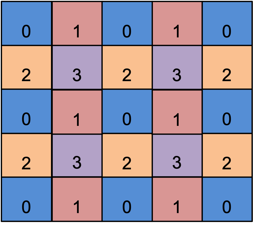
We partition the mesh elements into four disjoint subsets shown by the colors and numbers so that within each subset no two elements share a vertex.
For completeness, the computation of the four element indexing arrays is:
//
// Gather the element indices for each color in a vector.
//
  std::vector< std::vector<int> > idx(4);

  for (int ie = 0; ie < Nelem_tot; ++ie) {
    int i = ie % Nelem;
    int j = ie / Nelem;
    if ( i % 2 == 0 ) {
      if ( j % 2 == 0 ) {
        idx[0].push_back(ie);
      } else {
        idx[2].push_back(ie);
      }
    } else {
      if ( j % 2 == 0 ) {
        idx[1].push_back(ie);
      } else {
        idx[3].push_back(ie);
      }
    }
  }
RAJA Parallel Variants
To implement the vertex sum calculation using RAJA, we employ
RAJA::TypedListSegment iteration space objects to enumerate the mesh
elements for each color and put them in a RAJA::TypedIndexSet object.
This allows us to execute the entire calculation using one RAJA::forall
call.
We declare a type alias for the list segments to make the code more compact:
using SegmentType = RAJA::TypedListSegment<int>;
Then, we build the index set:
  RAJA::TypedIndexSet<SegmentType> colorset;

  colorset.push_back( SegmentType(&idx[0][0], idx[0].size(), host_res) );
  colorset.push_back( SegmentType(&idx[1][0], idx[1].size(), host_res) );
  colorset.push_back( SegmentType(&idx[2][0], idx[2].size(), host_res) );
  colorset.push_back( SegmentType(&idx[3][0], idx[3].size(), host_res) );
Note that we construct the list segments using the arrays we made earlier to partition the elements. Then, we push them onto the index set.
Now, we can use a two-level index set execution policy that iterates over the segments sequentially and executes each segment in parallel using OpenMP multithreading to run the kernel:
  using EXEC_POL1 = RAJA::ExecPolicy<RAJA::seq_segit,
                                     RAJA::omp_parallel_for_exec>;

  RAJA::forall<EXEC_POL1>(colorset, [=](int ie) {
    int* iv = &(e2v_map[4*ie]);
    areav[ iv[0] ] += areae[ie] / 4.0 ;
    areav[ iv[1] ] += areae[ie] / 4.0 ;
    areav[ iv[2] ] += areae[ie] / 4.0 ;
    areav[ iv[3] ] += areae[ie] / 4.0 ;
  });
The execution of the RAJA version is similar to the C-style OpenMP variant shown earlier, where we executed four OpenMP parallel loops in sequence, but the code is more concise. In particular, we execute four parallel OpenMP loops, one for each list segment in the index set. Also, note that we do not have to manually extract the element index from the segments like we did earlier since RAJA passes the segment entries directly to the lambda expression.
Here is the RAJA variant where we iterate over the segments sequentially, and execute each segment in parallel via a CUDA kernel launched on a GPU:
  using EXEC_POL2 = RAJA::ExecPolicy<RAJA::seq_segit,
                                     RAJA::cuda_exec<CUDA_BLOCK_SIZE>>;

  RAJA::forall<EXEC_POL2>(cuda_colorset, [=] RAJA_DEVICE (int ie) {
    int* iv = &(e2v_map[4*ie]);
    areav[ iv[0] ] += areae[ie] / 4.0 ;
    areav[ iv[1] ] += areae[ie] / 4.0 ;
    areav[ iv[2] ] += areae[ie] / 4.0 ;
    areav[ iv[3] ] += areae[ie] / 4.0 ;
  });
The only differences here are that we have marked the lambda loop body with the
RAJA_DEVICE macro, used a CUDA segment execution policy, and built a new
index set with list segments created using a CUDA resource so that the indices
live in device memory.
The RAJA HIP variant, which we show for completeness, is similar:
  using EXEC_POL3 = RAJA::ExecPolicy<RAJA::seq_segit,
                                     RAJA::hip_exec<HIP_BLOCK_SIZE>>;

  RAJA::forall<EXEC_POL3>(hip_colorset, [=] RAJA_DEVICE (int ie) {
    int* iv = &(d_e2v_map[4*ie]);
    d_areav[ iv[0] ] += d_areae[ie] / 4.0 ;
    d_areav[ iv[1] ] += d_areae[ie] / 4.0 ;
    d_areav[ iv[2] ] += d_areae[ie] / 4.0 ;
    d_areav[ iv[3] ] += d_areae[ie] / 4.0 ;
  });
The main difference for the HIP variant is that we use explicit device memory allocation/deallocation and host-device memory copy operations.